The enzyme-linked immunosorbent assay (ELISA) is a sensitive technique for determining the concentration of a protein in a liquid sample. When performing ELISAs, three different data outputs can be generated:
• Qualitative. An ELISA can be used to determine whether the protein of interest is found within a particular sample by comparing the sample to a blank well or a sample that does not contain the target protein.
• Semi-quantitative. Samples can be compared to one another to determine the relative amount of protein within each sample, as the intensity of signal is proportional to the concentration of the target protein.
• Quantitative. The amount of target protein within a sample can be precisely determined by setting up a standard curve of known target protein concentrations using purified antigen.
The preparation of the ELISA standard curve is critical in accurate sample quantification. This is a brief guide to preparing a standard curve and using the standard curve to quantify protein amounts.
Preparing the Standard Curve
Choice of standard
The standard curve should be prepared using purified protein. Some companies sell purified proteins that are suitable with ELISA assays. Purchased ELISA kits should contain a standard.
If purified protein is not available, then recombinant protein can be semi-purified in the lab and the concentration determined by HPLC.
Standard curve range
Typically, an ELISA measures protein concentrations in the range of 0.1-1 fmole or 0.01-0.1 ng, however this is dependent on the antibody-antigen interaction. Therefore, a classic standard curve ranges from 0-1000 pg/ml, although some can go as high as 3000 pg/ml if the samples to be measured are concentrated.
Reconstitute the standard
If the standard is supplied lyophilized, then it must be reconstituted prior to first use. To reconstitute the standard:
-
Spin the tube to collect all powder on the bottom.
-
Add the appropriate volume of standard diluent (the same diluent should be used for dilution of any samples).
-
Mix and let sit for 5 minutes at room temperature.
-
Mix again and aliquot the stock sample into single-use vials.
-
Freeze remaining standard solution at -20°C or below.
Serial dilutions
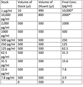
A standard curve is prepared by making serial dilutions of the protein standard within a range of concentrations near the expected concentrations of the unknown samples. An example of a dilution series for a standard curve ranging from 0-1000 pg/ml is given in Table 1 .
Table 1: Example Dilution Series for Standard Curve

*Not used in the assay.
To make the dilutions, use the following guidelines:
-
Make two- or three-fold dilutions.
-
Do not make dilutions that require pipetting a small amount of volume (2 ųl or less).
-
Avoid making large, single step dilutions. If the dilution is <1:1000, use two steps.
-
Prepare enough of each dilution to run in duplicate or triplicate.
-
Always include a background, negative control sample containing sample diluent.
-
Make dilutions fresh just before use.
-
Make all dilutions in tubes that do not absorb protein (polypropylene or glass; i.e. do not make dilutions in microplate).
-
Always use a fresh pipet tip for each dilution.
-
Mix each dilution well but avoid creating bubbles or foaming.
Prepare a new standard curve for every experiment and each plate
A standard curve run at different times will not have the same OD values for each dilution. This is due to operator differences and slight differences in pipetting, incubation times and temperature. Therefore, a new standard curve should be prepared for every experiment. Likewise, if analyzing more than one plate in an experiment, each plate should contain its own standard curve.
Using the Standard Curve to Quantify Samples
Once the intensity of each well has been measured on the plate reader, calculate the average absorbance values for each duplicate/triplicate sample. Then generate a standard curve by graphing the mean absorbance for each sample (x-axis) vs. the standard concentration (y-axis). Typically, a standard curve will have a sigmoidal shape in which the higher concentrations of standard dilutions will reach a plateau in absorbance.
Find the portion of the curve that is linear and draw the best-fit trendine for the data (many ELISA plate readers have built-in programs for generating and analyzing standard curves or you can use Microsoft Excel, or similar graphing software). Use the computer software to generate the equation of the line (i.e. y=mx + b; m= slope of the line and b= y intercept) and the R2 value. The R2 value is an indication of how closely the data fit the trendline. An R2 value of 1 is perfect.
Calculate the concentration of each sample by using the average of the duplicate/triplicate samples for x in the equation.
If the concentration of the sample exceeds the highest point of the curve or does not lie within the linear range of the curve, then dilute the sample prior to measurement. If a diluted sample is used, remembered to multiply by the dilution factor to obtain the final value.
Photo courtesy of Thomas Leth-Olsen.


